Single Object Detection

Intro

Hola ! | : )
How are you doing?

Sooo today, I'll be talking about how to build a single object detection model in pytorch.

But first of, let's briefly talk about single object detection:
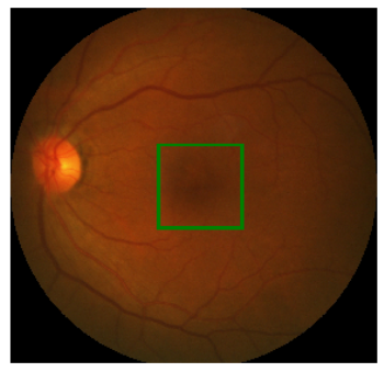
You see my child, single object detection is the process of finding the location of a specific object in an image. As opposed to multi-object detection, where we would be trying to find the location of different objects in an image.
The location of an object in an image, is usually defined with a bounding box (drawing a square around the object we want to located).

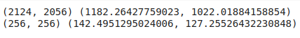
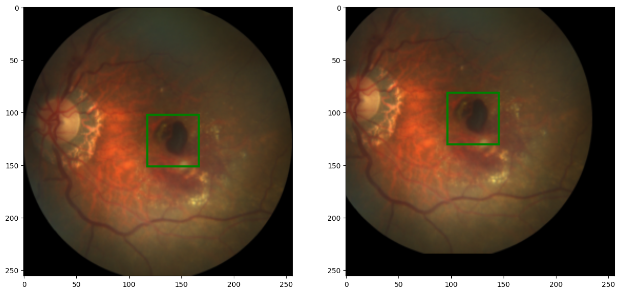
In this project we would build a model that can determine the location of the fovea in different eye images. So consequently, a fovea would be represented with (green) bounding boxes like so:

Load in Da Data

Now that we've established that, Let's load in DA DATAAAA:

The data we would use is the iChallenge-AMD dataset. You can get it from here.

When you've downloaded the dataset, upload it to google colab (or what ever platform you're using).

Now we have to make a directory for the dataset, and unzip the dataset into that directory:

!mkdir ./data
!unzip ./AMD-Training400.zip -d ./data
!unzip ./DF-Annotation-Training400.zip -d ./data

And with that ladies and gentlemen, we have loaded in da datatataaaa.

Let's Check out the dataset

We have an .xlsx file called Fovea_location.xlsx we should check that out:

import os
import pandas as pd

path2data = './data'
path2labels = os.path.join(path2data, 'Training400', 'Fovea_location.xlsx')

labels_df = pd.read_excel(path2labels, index_col='ID')
labels_df.head()

This is the output:

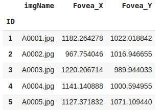
From this we can see that the Fovea_location.xlsx file contains the image name, and the (x, y) co-ordinates of the fovea in each image in the dataset.

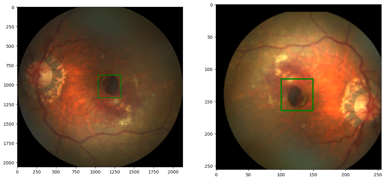
Now let's plot some images from the dataset:

To do this, we would need to build some functions to help us load images from their directories, and plot the said images

from PIL import Image, ImageDraw
import matplotlib.pylab as plt

def load_img_label(labels_df, id_):
	imgName = labels_df['imgName']
	if imgName[id_][0] == 'A':
		prefix = 'AMD'
	else:
		prefix = 'Non-AMD'

	fullpath2img = os.path.join(path2data, 'Training400', prefix, imgName[id_])
	img = Image.open(fullpath2image)
	x = labels_df['Fovea_X'][id_]
	y = labels_df['Fovea_Y'][id_]
	label = (x, y)
	return img, label

def show_img_label(img, label, w_h=(25, 25), thickness=2):
	draw = ImageDraw.Draw(img)
	cx, cy = label
	w, h = w_h
	draw.rectangle(((cx-w, cy-h), (cx+w, cy+h)), outline='green', width=thickness)
	plt.imshow(np.asarray(img))

In the first function load_img_label:

• We first get the prefix of the image we want to load from the image name check here for more info.
• Next we would create a oath to the image we want to load, and then load the image using the Image class from PILLOW
• Then we would get our label (x, y co-ordinates) for the image form the labels_df dataframe, and then return the image and label

**In the second function show_img_label:

• We first draw the image using the ImageDraw class from PILLOW, and consequently create an ImageDraw.Draw object for the image
• Then we get the center location of the fovea (the label), and store them in cx and cy (center x, center y)
• After this we would define the height and width we want our bounding box to have, as in w and h
• Then we use these values to draw our bounding box using the draw.rectangle() method which collects four points to define the box like so ((x0, y0), (x1, y1)), the outline which is green and the width (thickness) of the outline for the rectangle.
• Finally, we plot the image, together with the bounding box using the plt.imshow() method

Now that we've written these functions, we can use them like so:

import numpy as np

np.random.seed(2019)

plt.rcParams['figure.figsize'] = (15, 9)
plt.subplots_adjust(wspace=0, hspace=0.3)
nrows, ncols = 2, 3

imgName = labels_df['imgName']
ids = labels_df.index

rndIds = np.random.choice(ids, nrows*ncols) #get index of random images from labels_df

for i, id_ in enumerate(rndIds):
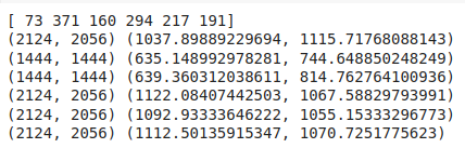
	img, label = load_img_label(labels_ds, id_)
	print(img.size, label)
	plt.subplot(nrows, ncols, i+1)
	show_img_label(img, label, w_h=(150, 150), thickness=20)
	plt.title(imgName[id_])

code output:

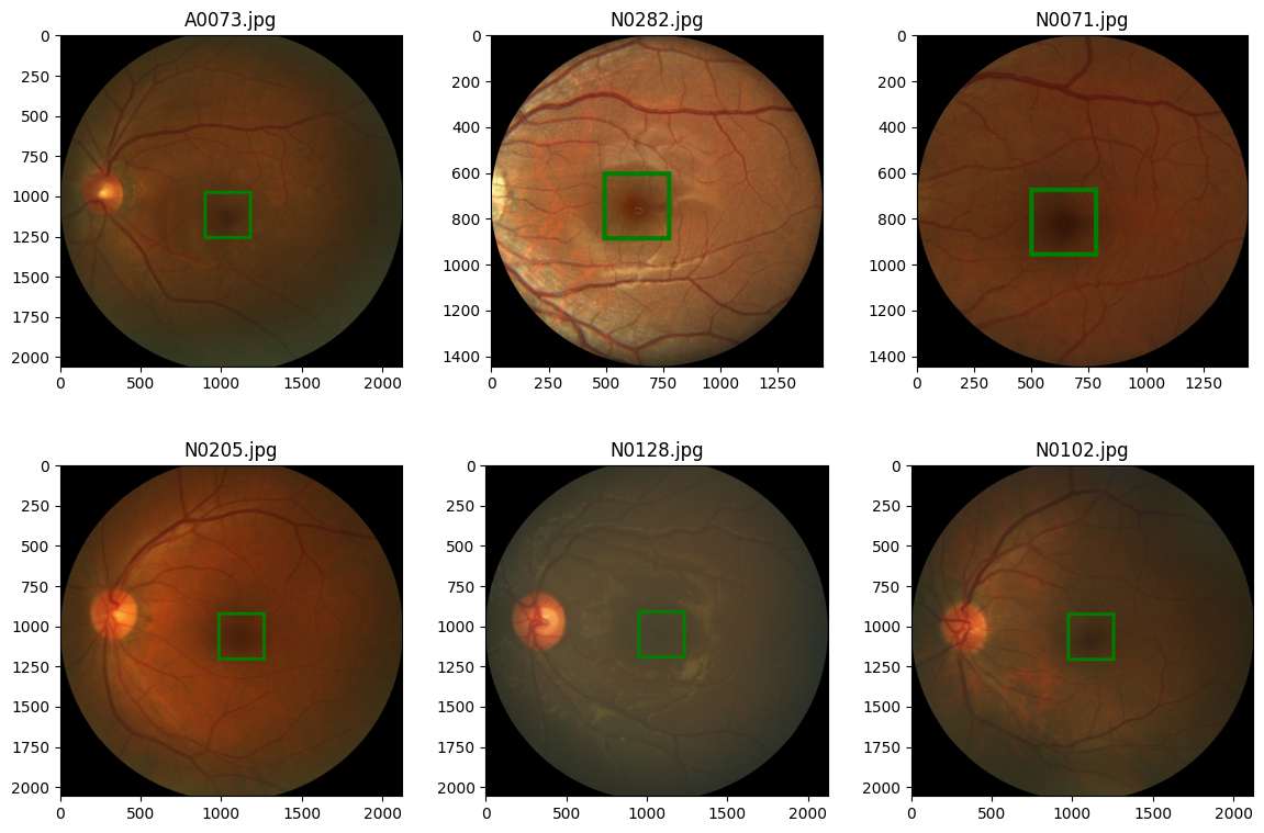
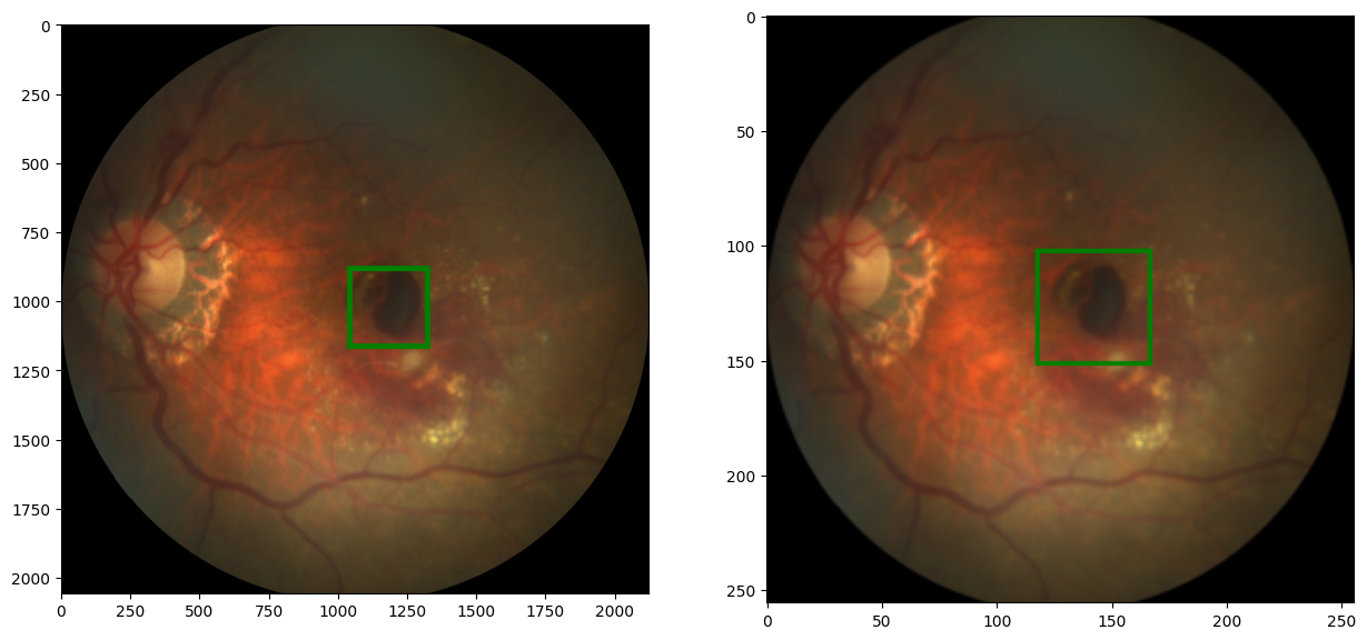
Notice that the images are of different sizes, this is a no no, when we go by the books, consequently, we would have to resize the image. And while we are at that we might as well create functions to help up augment the images.

Data Augmentation / Transformation

The transformation techniques we would be implementing are:

• resize image
• horizontal flip
• vertical flip
• shift

Let's get to it : )
PS I would use comments directly to explain the code snippets

Resizing Image

import torchvision.transforms.functional as TF

def resize_img_label(image, label=(0,0), target_size=(256, 256)):
	image_new = TF.resize(image, target_size) #resize image to target size
	
	original_width, original_height = image.size
	target_width, target_height = target_size
	cx, cy = label
	#resize label to target size. using simple algebra brah (lol)
	label_new = cx/original_width*target_width, cy/original_height*target_height

	return image_new, label_new

#test function
img, label = load_img_label(labels_df, 1) #load first image
print(img.size, label)

img_resize, label_resize = resize_image_label(img, label)
print(img_resize.size, label)

#plot images
plt.subplot(1, 2, 1)
show_img_label(img, label, w_h=(150, 150), thickness=20)
plt.subplot(1, 2, 2)
show_img_label(img_resize, label_resize)

code output:

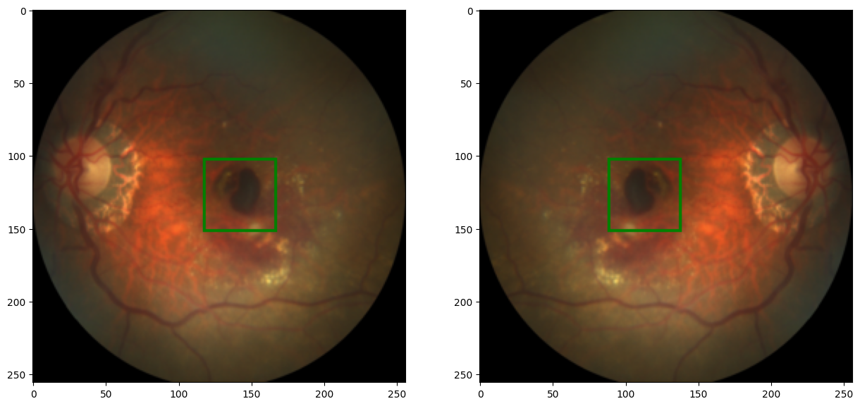
Horizontal Flip

def random_hflip(image, laebl):
	w, h = image.size
	x, y = label
	image = TF.hflip(image) #flip image using TF.hflip inbuilt function
	label = w-x, y 
	# since we are flipping horizontally, we have to update the x value of the label to correspond with the new image
	return image, label

#test function
img, label = load_img_label(labels_df, 1)
img_r, label_r = resize_img_label(img, label)
image_fh, label_fh = random_hflip(img_r, label_r)

#plot images
plt.subplot(1, 2, 1)
show_img_label(img_r, label_r)
plt.subplot(1, 2, 2)
show_img_label(img_fh, label_fh)

code output:

Vertical Flip

def random_vflip(image, label):
	w, h = image.size
	x, y = label

	image = TF.vflip(image) #flip image using TF.vflip inbuilt function
	label = x, w-y
	# since we are flipping vertically, we have to update the y value of the label to correspond with the new image
	return image, label

#test function
img, label = load_img_label(labels_df, 7)
img_r, label_r = resize_img_label(img, label)
img_fv, label_fv = random_vflip(img_r, label_r)

#plot images
plt.subplot(1, 2, 1)
show_img_label(img_r, label_r)
plt.subplot(1, 2, 2)
show_img_label(img_fv, label_fv)

code output:

Image Shift

import numpy as np
np.random.seed(1)

def random_shift(image, label, max_translate=(0.2, 0.2)):
	w, h = image.size
	max_t_w, max_t_h = max_translate #the maximum amount of shift that can be mae to the image
	cx, cy = label
	trans_coef = np.random.rand() * 2 - 1
	w_t = int(trans_coef * max_t_w * w)
	h_t = int(trans_coef * max_t_h * h)
	#translate (shift) the image using the TF.affine() function.
	image = TF.affine(image, translate=(w_t, h_t), shear=0, angle=0, scale=1)
	#update label value to correspond with translated image
	label = cx + w_t, cy + h_t
	return image, label

#test function
img, label = load_img_label(labels_df, 1)
img_r, label_r = resize_img_label(img, label)
img_t, label_t = random_shift(img_r, label_r, max_translate=(.5, .5))

#plot graph
plt.subplot(1, 2, 1)
show_img_label(img_r, label_r)
plt.subplot(1, 2, 2)
show_img_label(img_t, label_t)

code output:

Excellent ! Now we can combine all these function into a single function, to transform each image in our dataset:

import random
np.random.seed(0)
random.seed(0)

def transformer(image, label, params):
	image, label = resize_img_label(image, label, params['target_size'])
	
	if random.random() < params['p_hflip']:
		image, label = random_hflip(image, label)
	if random.random() < params['p_vflip']:
		image, label = random_vflip(image, label)
	if random.random() < params['p_shift']:
		image, label = random_shifti(image, label, params['max_translate'])
	if random.random() < params['p_brightness']:
		brightness_factor= 1 + (np.random.rand() * 2-1) * params['brightness_factor']
		image = TF.adjust_brightness(image, brightness_factor)
	if random.random() < params['p_contrast']:
		contrast_factor = 1 + (np.random.rand() * 2 - 1) * params['contrast_factor']
		image = TF.adjust_contrast(image, contrast_factor)
	if random.random() < params['p_gamma']:
		gamma = 1 + (np.random.rand() * 2 - 1) * params['gamma']
		image = TF.adjust_gamma(image, gamma)
	if params['scale_label']:
		label - scale_label(label, params['target_size'])

	image = TF.to_tensor(image)
	return image, label

#test function
img, label = load_img_label(labels_df, 1)

params={
	"target_size" : (256, 256),
	"p_hflip" : 1.0,
	"p_vflip" : 1.0,
	"p_shift" : 1.0,
	"max_translate": (0.5, 0.5),
	"p_brightness": 1.0,
	"brightness_factor": 0.8,
	"p_contrast": 1.0,
	"contrast_factor": 0.8,
	"p_gamma": 1.0,
	"gamma": 0.4,
	"scale_label": False,
}

img_t, label_t = transformer(img, label, params)

#plot output
plt.subplot(1, 2, 1)
show_img_label(img, label, w_h=(150, 150), thickness=10)
plt.subplot(1, 2, 2)
show_img_label(TF.to_pil_image(img_t),label_t)

output:

Superb!
The transform function basically takes in a dictionary object, containing probabilities of the transformations to occur, and then simply pass the image into our transformation functions, to transform the image. I also went ahead to add some extra transformations; brightness, contrast, gamma, and label scaling. As a result, you'll notice that the transformed image here is "brighter" that the original one.

Label scaling is super important more especially when it comes to object detection tasks. What the function does is to scale our label, to the range of [0, 1] using this function:

def scale_label(label, target_size):
	div = [ai/bi for ai, bi in zip(label, target_size)]
	return div

We should also have a rescale_label function in case we want to get the original values of the label:

def rescale_label(label, target_size):
	div = [ai*bi for ai, bi in zip(label, target_size)]
	return div

Now that we're done with image transformation, we should create our custom dataset class : )

Create Custom Dataset Class

Okay so to put simply, a dataset in pytorch is a class that provides an interface to access and retrieve data when training and evaluating a model. It acts as a bridge between the raw data and the model, this helps us to organize, preprocess and load the data efficiently.
To create our dataset, we would use the Dataset class from torch.utils.data we would override the __init__ and the __getitem__ functions.

from PIL import Image
from torch.utils.data import Dataset

class AMD_Dataset(Dataset):
	def __init__(self, path2data, transform, trans_params):
		path2labels = os.path.join(oath2data, 'Training400', 'Fovea_location.xlsx')
		labels_df = pd.read_excel(path2labels, index_col='ID')
		
		self.labels = labels_df[['Fovea_X', 'Fovea_Y']].values
		self.imgName = labels_df['imgName']
		self.ids = labels_df.index
		
		self.fullpath2img = [0]*len(self.ids)
		for id_ in self.ids:
			if self.imgName[id_][0] = 'A':
				prefix = 'AMD'
			else:
				prefix = 'Non-AMD'
			self.fullpath2img[id_-1] = os.path.join(path2data, 'Training400', prefix, self.imgName[id_])
		
		self.transform = transform
		self.trans_params = trans_params

	def __len__(self):
		return len(self.labels)
	
	def __getitem__(self, idx):
		image = Image.open(self.fullpath2img[idx])
		label = self.labels[idx]
		image, label = self.transform(image, label, self.trans_params)
		
		return image, label

Sooooo, what we've done here is to:

• create the important attributes for our dataset class in the __init__ method, the attributes are:
  • the labels. (self.labels)
  • the full path to the image. (self.fullpath2image)
  • the transform attribute with is basically going to be our transform function. (self.transform)
  • the transform parameters attribute, which is the dictionary object we would pass into the transform attribute when calling it. (self.trans_params)
• implement the __len__ function to return the length of the dataset
• implement the __getitem__ function to return a transformed Image and it's corresponding label at a given index.

Now we would create our training and validation dataset. To do this, we would define the transformation parameters, split the dataset and then use the Subset class to load the datasets.

from sklearn.model_selection import ShuffleSplit
from torch.utils.data import Subset

#define tranformation parameters
trans_params_train = {
	'target_size': (256, 256),
	'p_hflip': 0.5,
	'p_vflip': 0.5,
	'p_shift': 0.5,
	'max_translate': (0.2, 0.2),
	'p_brightness': 0.5,
	'brightness_factor': 0.2,
	'p_contrast': 0.5,
	'contrast_factor': 0.2,
	'p_gamma': 0.5,
	'gamma': 0.2,
	'scale_label': True
}

trans_params_val = {
	'target_size': (256, 256),
	'p_hflip': 0.0,
	'p_vflip': 0.0,
	'p_shift': 0.0,
	'max_translate': (0.0, 0.0),
	'p_brightness': 0.0,
	'brightness_factor': 0.0,
	'p_contrast': 0.0,
	'contrast_factor': 0.0,
	'p_gamma': 0.0,
	'gamma': 0.0,
	'scale_label': True
}

#split dataset into training and validation
amd_ds1 = AMD_dataset(path2data, transformer, trans_params_train)
amd_ds2 = AMD_dataset(path2data, tranformer, trans_params_val)

sss = ShuffleSplit(n_splits=1, test_size=0.2, random_state=0)

indices = range(len(amd_ds1))

for train_index, val_index in sss.split(indices):
	print(len(train_index))
	print('-'*10)
	print(len(val_index))

train_ds = Subset(amd_ds1, train_index)
val_ds = Subset(amd_ds2, val_index)

Excellent!!

Now you might be wondering why I created 2 different amd_ds classes this is because the training and validation dataset has different transformation parameters (the only transformation going to happen in the validation dataset is image_resize and label_scaling). So we create 2 dataset classes (initially) with different transformation parameters.

We use the Subset class to divide the original dataset (amd_ds1 and amd_ds2) classes in to the final train_ds and val_ds dataset.

We should plot some images from the dataset classes (#sanity_check)

import matplot.pyplot as plt
%matplotlib inline
np.random.seed(0)

def show(img, label=None):
	npimg = img.numpy().transpose((1, 2, 0))
	plt.imshow(npimg)
	if label is not None:
		label = rescale_label(label, img.shape[1:])
		x, y = label
		plt.plot(x, y, 'b+', markersize=20)

plt.figure(figsize=(5, 5))
for img, label in train_ds:
	show(img, label)
	break

plt.figure(figsize=(5, 5))
for img, label in val_ds:
	show(img, label)
	break

output:

• train_ds
  

• val_ds
  

Hehe : )

Now that our datasets has been setup successfully, we can finally push them into a dataloader:

from torch.utils.data import DataLoader

train_dl = Dataloader(train_ds, batch_size=8, shuffle=True)
val_dl = Dataloader(val_ds, batch_size=16, shuffle=False)

Let's checkout the dataloader:

for img_b, label_b in train_dl:
	print(img_b.shape, img_b.type)
	print(label_b)

output:

torch.Size([8, 3, 256, 256]) <built-in method type of Tensor object at 0x7db4f273a0c0> 

[tensor([0.6728, 0.5278, 0.4779, 0.5037, 0.6933, 0.5131, 0.4818, 0.5169], dtype=torch.float64), 
tensor([0.5979, 0.5398, 0.5221, 0.4609, 0.6326, 0.5074, 0.5071, 0.5203], dtype=torch.float64)]

This look's mostly correct, but there's a small issue with the shape of the labels in a batch. Here we have a list containing two tensors. The first tensor contains values that show the x-coordinate of the fovea for each image in the batch, and the second tensor contains values that represents the y-coordinate, in other words we have something like this :
[(x1, x2, x3, ...), (y1, y2, y3, ...)] .
We don't want this, what would be better would be having a tensor that contains x and y coordinates in pairs, like so [(0.6728, 0.5979), (0.5278, 0.5398), (x3, y3), ...]. To do this, we can use the torch.stack() method. We would implement this in our training loop, but here's how it works.

Now that we're done with this, let's build da model !!!

Building Da Model

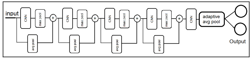
We'll build a typical model that has several convolutional and pooling layers, that would receive our resized RGB image, and them return two linear outputs, that represents the (x, y) coordinates of the fovea location.
Here's how the model looks like : )

Let's get cooking.

So to build our model in pytorch, we would need to implement two methods in the class

• The __init__() method
• The forward() method

Let's implement the __init__() method first :

import torch.nn as nn
import torch.nn.functional as F

class Net(nn.Module):
	def __init__(self, params):
		super(Net, self).__init__()
		
		C_in, H_in, W_in = params['input_shape']
		init_f = params['initial_filters']
		num_outputs = params['num_outputs']
		
		self.conv1 = nn.Conv2d(C_in, init_f, kernel_size=3, stride=2, padding=1)
		self.conv2 = nn.Conv2d(init_f+C_in, 2*init_f, kernel_size=3, padding=1)
		self.conv3 = nn.Conv2d(3*init_f+C_in, 4*init_f, kernel_size=3, padding=1)
		self.conv4 = nn.Conv2d(7*init_f+C_in, 8*init_f, kernel_size=3, padding=1)
		self.conv5 = nn.Conv2d(15*init_f*C_in, 16*init_f, kernel_size=3, padding=1)
		
		self.fc1 = nn.Linear(16*init_f, num_outputs)

In this method, we basically initialized (instantiated), the model's components;

• Firstly, we have C_in, H_in, W_in which represents the number of channels, the height and the width of the picture being passed into the image. For our task, the initial color channel value is three (RGB).
• The second variable init_f represents the number of initial filters, that we would use in the first convolutional layer
• We also have the num_outputs variable, which represents the shape of the output variable: the (x, y) coordinate of the fovea location.
• After that we have our convolutional layers. the parameters of the nn.Conv2d layers are:
  • number of input channels
  • number of filters to apply to each channel
  • the kernel size
  • the stride of the kernel
  • and the padding
• And finally, our fully connected layer self.fc1, which is the last layer that returns the actual (x, y) coordinates of fovea location.

Now let's cook up the forward method:

class Net(nn.Module):
	def __init__(self, params):
		...
	
	def forward(self, x):
		identity = F.avg_pool2d(x, 4, 4)
		x = F.relu(self.conv1(x))
		x = F.max_pool2d(x, 2, 2)
		x = torch.cat((x, identity), dim=1)
		
		identity = F.avg_pool2d(x, 2, 2)
		x = F.relu(self.conv2(x))
		x = F.max_pool2d(x, 2, 2)
		x = torch.cat((x, identity), dim=1)
		
		identity = F.avg_pool2d(x, 2, 2)
		x = F.relu(self.conv3(x))
		x = F.max_pool2d(x, 2, 2)
		x = torch.cat((x, identity), dim=1)
		
		identity = F.avg_pool2d(x, 2, 2)
		x = F.relu(self.conv4(x))
		x = F.max_pool(x, 2, 2)
		x = torch.cat((x, identity), dim=1)
		
		x = F.relu(self.conv5(x))
		x = F.adaptive_avg_pool2d(x, 1)
		x = x.reshape(x.size(0), -1)
		
		x = self.fc1(x)
		return x

In here we basically implemented what we have in the model diagram above. Which is basically:

• Getting an identity matrix by average_pooling the x value
• passing the x value into the convolutional layer, using the relu activation function
• Getting a max_pool matrix from the output of the convolutional layer
• And then concatenating the the average_pool matrix (identity) and the max_pool matrix, to form a new feature, using the torch.cat() method.
• We do this until we reach the final convolutional layer, and then we pass the features, into the fully connected layer, which returns the final value we take as our output.

As easy as that [- _ -]

Finally, let's instantiate our model

params_model = {
				'input_shape': (3, 256, 256),
				'initial_filters': 16,
				'num_outputs': 2
}

model = Net(params_model)

#push to GPU if available
if torch.cuda.is_available():
	device = torch.device('cuda')
	model = model.to(device)

print(model)

output:

Net( (conv1): Conv2d(3, 16, kernel_size=(3, 3), stride=(2, 2), padding=(1, 1))
	 (conv2): Conv2d(19, 32, kernel_size=(3, 3), stride=(1, 1), padding=(1, 1))
	 (conv3): Conv2d(51, 64, kernel_size=(3, 3), stride=(1, 1), padding=(1, 1)) 
	 (conv4): Conv2d(115, 128, kernel_size=(3, 3), stride=(1, 1), padding=(1, 1)) 
	 (conv5): Conv2d(243, 256, kernel_size=(3, 3), stride=(1, 1), padding=(1, 1)) 
	 (fc1): Linear(in_features=256, out_features=2, bias=True) 
	 )

The next step is to define our loss function, optimizer and our performance metric which is going to be IOU aka. Jaccard Index.

Defining Loss Function, Optimizer, and Performance Metric

For this task the loss function we would use is the Smooth-L1 Loss, it's a regularly used loss function for object detection tasks. Smoothed-L1 loss squares the term if the absolute element-wise error falls below 1, and returns the L1 term if the error is above 1. in other words, this loss is useful in scenarios where you want your model to be less sensitive to small errors, but still penalize larger error effectively. (Just like in our case)

The optimizer we would for this task, is our good old Adam optimizer.

from torch import optim
from torch.optim.lr_scheduler import ReduceLROnPlateau
import torchvision

loss_func = nn.SmoothL1Loss(reduction='sum')
opt = optim.Adam(model.parameters(), lr=3e-4)

def get_lr(opt):
	for param_group in opt.param_groups:
		return param_group['lr']

lr_scheduler = ReduceLROnPlateau(opt, mode='min', factor=0.5, patience=20, verbose=1)

Now for the Performance metric, we would use is the Intersect over Union (IOU). it basically quantifies the overlap between the predicted bounding box and the ground truth bounding box.
This image shows how it works:

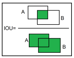
As you can see, it divides the Intersect of the 2 boxes, by their union. (hence the name Intersect over Union).

def cxcy_to_boundary_box(cxcy, w=50./256, h=50./256):
	w_tensor = torch.ones(cxcy.shape[0], 1, device=cxcy.device) * w
	h_tensor = torch.ones(cxcy.shape[0], 1, device=cxcy.device) * h

	cx = cxcy[:, 0].unsqueeze(1)
	cy = cxcy[:, 1].unsqueeze(1)
	
	boxes = torch.cat((cx, cy, w_tensor, h_tensor), -1)
	
	return torch.cat((boxes[:, :2] - boxes[:, 2:]/2,
					  boxes[:, :2] + boxes[:, 2:]/2), -1)

def metrics_batch(output, target): 
	output = cxcy_to_boundary_box(output)
	target = cxcy_to_boundary_box(target)
	iou = torchvision.ops.box_iou(output, target)
	return torch.diagonal(iou, 0).sum().item()

Here we have 2 functions;

• The first function cxcy_to_boundary_box converts (x, y) coordinates of the fovea location to boundary box format (x1, y1), (x2, y2). The function handles this for batches of data. That's why it looks all weird like that. It basically returns an array containing multiple (x1, y1), (x2, y2) values.
• The second function metrics_batch is where the IOU values are being calculated. We would pass in the ground truth (target) value and the model's output, convert these values to boundary box format, and then use pytorch's inbuilt .box_iou() method to calculate IOU values for each "output-target" pair in the batch, and then return the sum of the results.

It's finally time for the main training and validation loop

Defining the main training loop

Let's first cook up functions to handle calculating loss per batch, and loss per epoch.

def loss_batch(loss_func, output, target, opt=None):
	loss = loss_func(output, target)
	with torch.no_grad():
		metric_b = metrics_batch(output, target)
	if opt is not None:
		opt.zero_grad()
		loss.backward()
		opt.step()
	
	return loss.item(), metric_b

def loss_epoch(model, loss_func, dataset_dl, opt=None):
	running_loss = 0.0
	running_metric = 0.0
	len_data = len(dataset_dl.dataset)
	
	for xb, yb in dataset_dl:
		yb = torch.stack(yb, 1)
		yb = yb.type(torch.float32).to(device)
		output = model(xb.to(device))
		loss_b, metric_b = loss_batch(loss_func, output, yb, opt)
		running_loss += loss_b
		if metric_b is not None:
			running_metric += metric_b
	
	loss = running_loss/float(len_data)
	metric = running_metric/float(len_data)
	
	return loss, metric

• In the loss_batch function, we simply calculate the loss and metric (IOU) value for that batch, and update the model's weight based on the loss value.
• In the loss_epoch function, we try to calculate the loss and metric gotten for that epoch. To do this, we iterate the batches from the dataloader, get the loss and metric for each batch, using the loss_batch function and then aggregate all the losses and metrics from each batch to get our loss and metric for that epoch.

Now for our main training and validation loop:

import copy

def train_val(model, params):
	num_epochs = params['num_epochs']
	loss_func = params['loss_func']
	opt = params['opt']
	train_dl = params['train_dl']	
	val_dl = params['val_dl']	
	lr_scheduler = params['lr_scheduler']	
	path2weights = params['path2weights']
	
	loss_history = {
		'train': [],	
		'val': [] 
	}  
	
	metric_history = {
		'train': [],
		'val': []
	}
	
	best_model_wts = copy.deepcopy(model.state_dict())
	best_loss = float('inf')

	for epoch in range(num_epochs):
		current_lr = get_lr(opt)
		print(f'Epoch {epoch+1}/{num_epochs}, current_lr = {current_lr}')
		
		model.train()
		train_loss, train_metric = loss_epoch(model, loss_func, train_dl, opt)
		loss_history['train'].append(train_loss)
		metric_history['train'].append(train_metric)

		model.eval()
		with torch.no_grad():
			eval_loss, eval_metric = loss_epeoch(model, loss_func, val_dl)
			loss_history['val'].append(eval_loss)
			metric_history['val'].append(eval_metric)
		
		if eval_loss < best_loss:
			best_loss = eval_loss
			best_model_wts = copy.deepcopy(model.state_dict())
			torch.save(model.state_dict(), path2weights)
			print('Copied best model weights')
		
		lr_scheduler.step(eval_loss)
		if current_lr != get_lr(opt):
			print('Loading best model weights')
			model.load_state_dict(best_model_wts)
		
		print('train loss: %.6f, accuracy: %.2f'%(train_loss, 100*train_metric))
		print('eval loss: %.6f, accuracy: %.2f'%(eval_loss, 100*eval_metric))

	model.load_state_dict(best_model_wts)
	return model, loss_history, metric_history

This is typically what a regular training and validation loop looks like:

• First we initialise our necessary training and validation parameters
• The we start the epoch loop
• In the epoch loop, we train the model, and then evaluate the model's performance after the last training session is done; so it's like: train >> validate >> train >> validate
• After evaluating the model's performance, we check to see if the current eval loss is the best we've gotten, if it is, we store the model's weights
• Finally we update our learning rate scheduler, then we check if the new learning rate (gotten from lr_scheduler.step(eval_los)) is the different from the current learning rate, if it is, we load on the best recorded model weights, so that the model can use the new learning rate from the best state so far.
• After the loop is finished, we load the best model weights into the model, and then return the model, loss history and metric history.

It's finally time to train (omg I could cry rn lol):

Training the model

For this, all we have to do is to call the train_val function

path2models = "./models/"

if not os.path.exists(path2models):
	os.mkdir(path2models)

params_train = {
	"num_epochs": 100,
	"opt": opt,
	"loss_func": loss_func,
	"train_dl": train_dl,
	"val_dl": val_dl,
	"lr_scheduler": lr_scheduler,
	"path2weights": path2models+"weights_smoothl1.pt",
}

model, loss_hist, metric_hist = train_val(model,params_train)

Visualizing Training Results

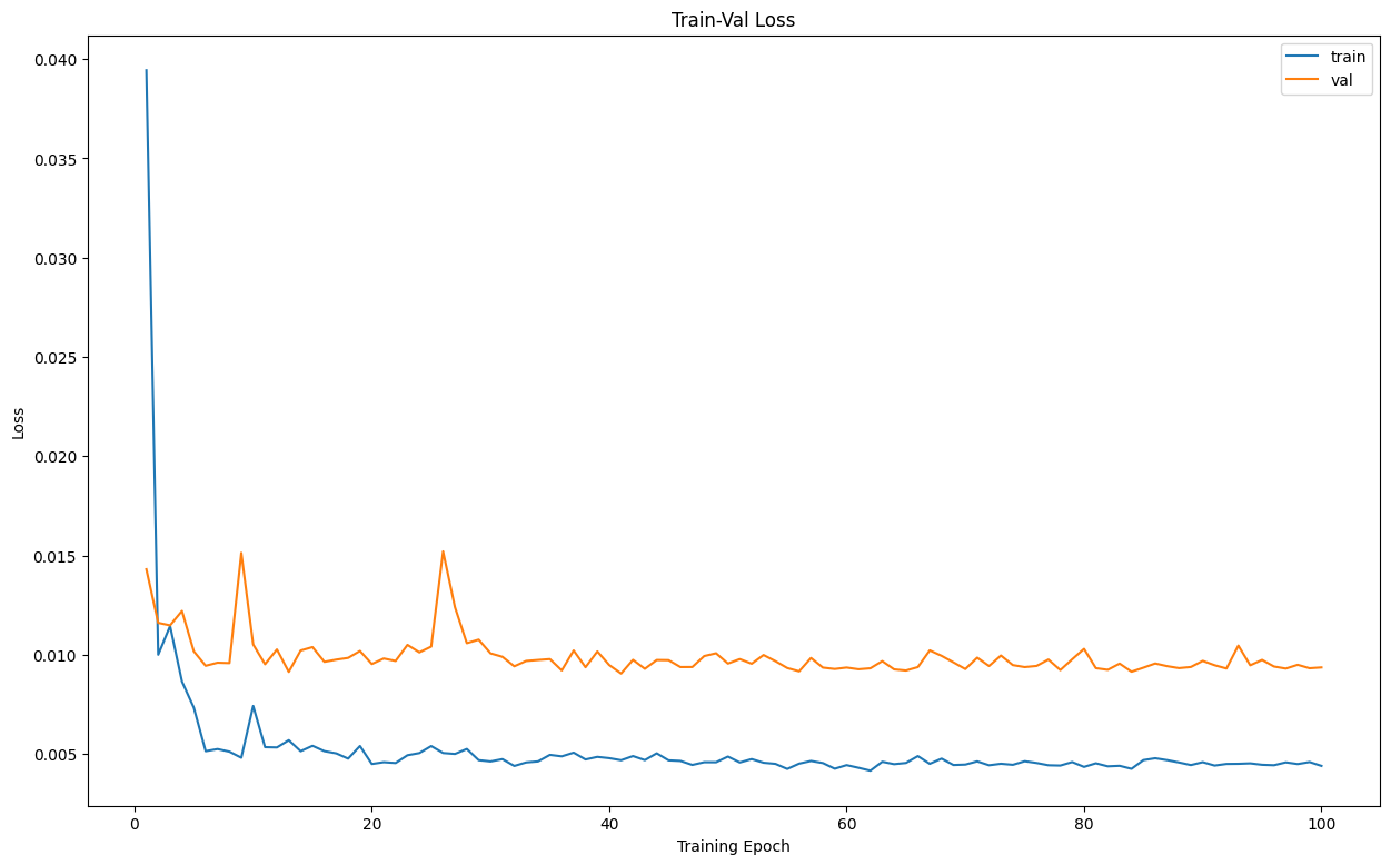
Let's first visualize the loss during training

num_epochs = params_train['num_epochs']

plt.title('Train-Val Loss')
plt.plot(range(1, num_epochs+1), loss_hist['train'], label='train')
plt.plot(range(1, num_epochs+1), loss_hist['val'], label='val')
plt.ylabel('Loss')
plt.xlabel('Training Epoch')
plt.legend()
plt.show()

Output:

And then visualize the training metrics

plt.title('Train-Val Accuracy')
plt.plot(range(1, num_epochs+1), metric_hist['train'], label='train')
plt.plot(range(1, num_epochs+1), metric_hist['val'], label='val')
plt.ylabel('Accuracy (IOU)')
plt.xlabel('Training Epoch')
plt.legend()
plt.show()

Output:

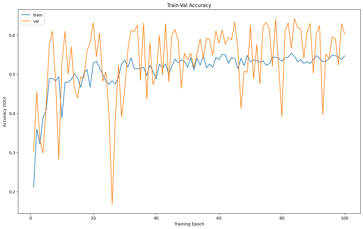
The plots have a good shape, the model's performance seems to be alright.
Typically, you would want a down trend in a loss plot, and an up trend in an accuracy plot, since our graphs seem to have that shape, we can say the model's performance is alright.

But I could argue, nothing would beat seeing the model in action when trying to measure performance : )
Let's do just that.

Model Deployment

To see the model's performance, we would load on the model and then make predictions on some test images, and then plot the predicted boundary box and the actual boundary box to see how well they over lap

params_model = {
	'input_shape': (3, 256, 256),
	'initial_filters': 16,
	'num_outputs': 2
}

model = Net(params_model)
model.eval()

if torch.cuda.is_available():
	device = torch.device('cuda')
	model = model.to(device)

path2weigths = '.../model_weights.pt' #make sure to add the actual path to the weights on your own machine
model.load_state_dict(torch.load(path2weights))

Now that we have loaded the model, we should create a function that would plot the test image together with the predicted label and target label:

from PIL import ImageDraw
import numpy as np
import torchvision.transforms.functional as tv_F
import matplotlib.pylab as plt

%matplotlib inline
np.random.seed(0)

def show_model_predictions(img, label1, label2, w_h=(25, 25)):
	label1 = rescale_label(label1, img.shape[1:])
	label2 = rescale_label(label2, img.shape[1:])
	img = tv_F.to_pil_image(img)
	
	w, h = w_h
	
	cx, cy = label1
	draw = ImageDraw.Draw(img)
	draw.rectangle(((cx-w, cy-h), (cx+w, cy+h)), outline='green', width=2)
	
	cx, cy, = label2
	draw.rectangle(((cx-w, cy-h), (cx+w, cy+h)), outline='red', width=2)  
	
	plt.imshow(np.asarray(img))

Sweet ! It's basically the same as the other image plot function we have above, the difference is just that this one would plot two boundary boxes.

Now let's get plotting:

rndInds = np.random.randint(len(val_ds), size=10)

plt.rcParams['figure.figsize'] = (15, 10)
plt.subplots_adjust(wspace=0.0, hspace=0.15)  

for i, rndi in enumerate(rndInds):
	img, label = val_ds[rndi]
	h, w = img.shape[1:]
	
	with torch.no_grad():
		label_pred = model(img.unsqueeze(0).to(device))[0].cpu()
		
	plt.subplot(2, 3, i+1)
	show_model_predictions(img, label, label_pred)
	label_bb = cxcy_to_boundary_box(torch.tensor(label).unsqueeze(0))
	label_pred_bb = cxcy_to_boundary_box(torch.tensor(label_pred).unsqueeze(0))
	iou = torchvision.ops.box_iou(label_bb, label_pred_bb)
	plt.title('%.2f'%iou.item())
	
	if i > 4:
		break

Output:

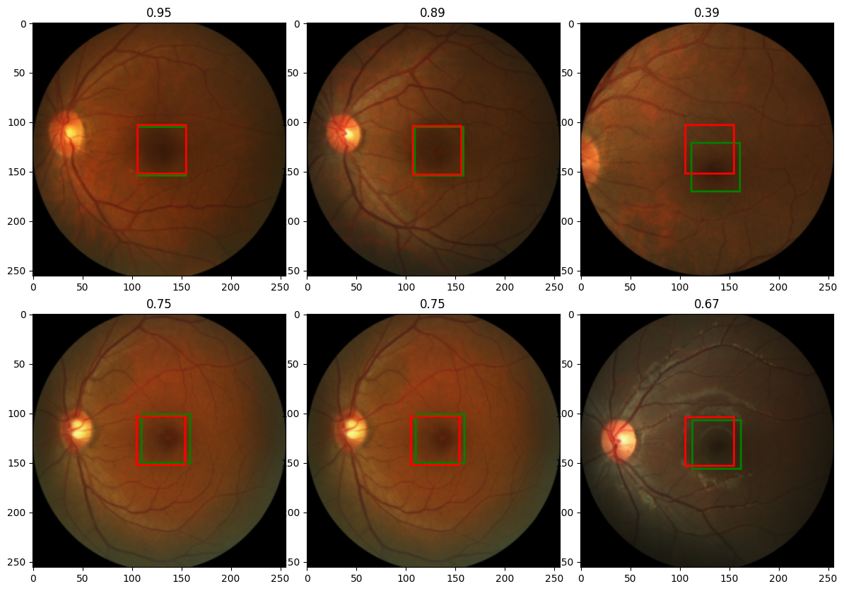
Excellent!!!
Note that the red boxes are the predicted boxes, while the green one are the target boundary boxes.
The value above the images, are the IOU values of the boundary boxes. An IUO value of 1.00 means perfect match of the boundary boxes.

And with that ladies and gents. We have come to the end of the journey.
What's next ??
Even I can't answer that yet lol

Fovea-Centralis

The fovea centralis is a small, central pit composed of closely packed cones in the eye. It is located in the center of the macula lutea of the retina

The fovea is responsible for sharp central vision (also called foveal vision), which is necessary in humans for activities for which visual detail is of primary importance, such as reading and driving.

PS: This is literally gotten from wikipedia, You do not really need to have a deep understanding on what a fovea is.

AMD-Dataset

There are 2 classes of images in this dataset, AMD and Non-AMD, this is only necessary to us, when we want to perform a classification task.

Image-Augmentation

Image Augmentation is a technique used to increase the size of training dataset in deep learning computer vision tasks. The aim is basically to introduce diversity and variability in the dataset. This helps the model generalize better to unseen data : )

torch.stack()

import torch
#first let's create a list that has a similar shape as our label_b
a = [torch.Tensor([1, 2, 3, 4, 5]), torch.Tensor([5, 4, 3, 2, 1])]

#now let's pair them together around axis 1
b = torch.stack(a, 1)

print(a)
print(b)

output:

[tensor([1., 2., 3., 4., 5.]), tensor([5., 4., 3., 2., 1.])] 

tensor([[1., 5.], 
	[2., 4.], 
	[3., 3.], 
	[4., 2.], 
	[5., 1.]])

Yup it's as easy as that : )