Multi-Class Image Classification
Recently, I've been learning how to use pytorch, mainly for computer vision tasks.
Today, I'll talk about how we can use pytorch for multi class image classification.
So first-off multi class image classification is a kind of computer vision task, where the aim is to identify an image, and group it to a single class, eg. classifying images of animals into categories like "dog" "cat" "dinosaur" "dragon" "unicorn" etc... In this case, each image belongs to only one class
Now, the dataset we're going to use is referred to as the "STL-10 dataset". The dataset consists of 10 classes which are shown below:
| Class Name | Class Label |
|---|---|
| Air plane | 0 |
| Bird | 1 |
| Car | 2 |
| Cat | 3 |
| Deer | 4 |
| Dog | 5 |
| Horse | 6 |
| Monkey | 7 |
| Ship | 8 |
| Truck | 9 |
The dataset consists of 5 000 training images, and 8 000 test images, which by extension means each class has 500 and 800 images for training and testing.
The images are RGB and their dimensions are 96x96. Also, conveniently, the dataset is available in pytorch, that we can access with the torchvision package.
You can get more info on the dataset here : )
NOW WE SHALL LOAD IN DA DATA !!!
open your python file (or notebook, anyone you like really, I personally would recommend a python notebook for this one though).
We would import the data like so:
from torchvision import datasets
from torchvision.transforms import transforms
import os

path_to_data = './data'

if not os.path.exists(path_to_data):
	os.mkdir(path_to_data)

data_transformer = transforms.Compose([transforms.ToTensor()])

#load the train data
train_ds = datasets.STL10(path_to_data, split='train', download=True, transform=data_transformer)

#load the test data
test0_ds = datasets.STL10(path_to_data, split='test', download=True, transforms=data_transformer)
So, what we have done here is to:
- first create the directory to store the dataset using the
os.mkdir()method - then we create a data transformer object. The aim of the transformer is to basically convert the images to tensors that's why you see the
transforms.ToTensor()there. - then we load the train and test dataset, specifying the data path, the split, and the transformer to apply to each image being downloaded
Now we have to split the test0_ds dataset into test and validation datasets.
To do this, we would use sklearn's StratifiedShuffleSplit like so:
from sklearn.model_selection import StratifiedShuffleSplit

sss = StratifiedShuffleSplit(n_splits=1, test_size=0.2, random_state=0)

indices = list(range(len(test0_ds)))
y_test0 = [y for _, y in test0_ds]

for test_index, val_index in sss.split(indices, y_test0):
	print((f'test: {test_index} val: {val_index}')
	print(len(val_index), len(test_index))
ok, so what we have basically done here is:
- create the
StratifiedShuffleSplitobject, with n_split set to 1, which simply means that the number of re-shuffling and splitting iterations done would be 1. - then we create an
indicesobject, that basically has the index of each image in thetest0_dsdataset - we also create a list
y_test0that contains the label for each image in thetest0_dsdataset - then we use a for-loop to get split the dataset into test and validate, which are stored in the
test_indexandval_indexvariables.
The indices and y_test0 objects are what has been passed into the StratifiedShuffleSplit object, which then returns 2 lists containing indexes of the images that belong to the test and validate datasets.
After getting the indexes, we would then create the actual ("X" and "y") datasets (the one that would contain the actual tensors and stuff). WE SHALL USE THE SUBSET CLASS FROM THE LAND OF torch.utils.data like so:
from torch.utils.data import Subset
import numpy as np

val_ds = Subset(test0_ds, val_index)
test_ds = Subset(test0_ds, test_index)

y_val = [y for _, y in val_ds]
y_test = [y for _, y in test_ds]

#check if the distribution of class labels is identical
import collections

counter_test = collections.Counter(y_test)
counter_val = collections.Counter(y_val)

print(counter_test)
print(counter_val)
So what we have done here is:
- use the
Subsetclass to create theval_dsandtest_dsdataset, by passing the originaltest0_dsdataset, and the list indexes for the datasets that has been created byStratifiedShuffleSplit - we then extract the labels for each of the datasets
- and we use the collections module to check the distribution of labels in the two datasets.
The output of the code should be:
Counter({6: 640, 0: 640, 4: 640, 5: 640, 9: 640, 2: 640, 3: 640, 1: 640, 7: 640, 8: 640})
Counter({2: 160, 8: 160, 3: 160, 6: 160, 4: 160, 1: 160, 5: 160, 9: 160, 0: 160, 7: 160})
As you can see the the amount of labels in both datasets are the same: 640 for the test dataset, and 160 for the validate dataset.
Now I'd like us to view some images from our dataset : )
To do this, we would create a function to help us plot the images. We would use matplotlib for this:
from torchvision import utils
import matplotlib.pyplot as plt

np.random.seed(0)

def show(img, y=None):
	npimg = img.numpy()
	npimg_tr = np.transpose(npimg, (1, 2, 0))
	plt.imshow(npimg_tr)
	if y is not None:
		plt.title(f'label: {str(y)}')

grid_size = 4
random_indexes = np.random.randint(0, len(train_ds), grid_size)

x_grid = [train_ds[i][0] for i in random_indexes]
y_grid = [train_ds[i][1] for i in random_indexes]

x_grid = utils.make_grid(x_grid, nrow=4, padding=1)

plt.figure(figsize(10, 10))
show(x_grid, y_grid)
What we have done in this code is:
- create the function
showto help us display the image, by first converting the tensors to a numpy array, and then transposing it, making the image to be in the right format for theply.imshow()method. - then we randomly picked images, and labels from the test data, and converted them to a grid, using the
torchvision.utils.make_grid()method, which collects the list of images selected, and then concatenate the images side-by-side following thenrowparameter (this is why we have 4 images on the plot). - After this we simply call the
showmethod, to display our images.
The original shape on the image tensors is [3, 96, 96] which represents:
[color_scheme (RGB), length (x), height (y)]
But this format is not what the plt.imshow() method expects. it expects an array in this format [lenght (x), height (y), color_scheme (RGB)].
As a result, we have to transpose the numpy array as seen in the show method.
the tuple (1, 2, 0) simply means convert the array with dimension [3, 96, 96] to [96, 96, 3]
i.e from (index-zero, index-one, index-two) to (index-one, index-two, index-zero)
This would be the output of the code.
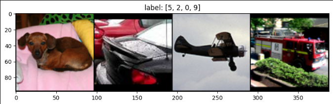
Hehe: "What tha dog doing??" lol
The next step is Image pre-processing : )
One of the things we would do is to normalize our image data. To normalize our data, simply means to make it so that the dataset has a mean of 0 and a standard deviation of 1. it is calculated like so:
normalized value = (original value − mean) / standard deviation
in our case, we would normalize each color channel, by calculating the the mean and std for each channel, and then normalizing them. we would do this first determining the mean RGB values, and then using the torchvision.transforms.transforms.Normalize() method to normalize the datasets like this:
meanRGB = [np.mean(x.numpy(), axis=(1, 2)) for x, _ in train_ds]
stdRGB = [np.std(x.numpy(), axis=(1, 2)) for x, _ in train_ds]

meanR=np.mean([m[0] for m in meanRGB])
meanG=np.mean([m[1] for m in meanRGB])
meanB=np.mean([m[2] for m in meanRGB])

stdR=np.mean([s[0] for s in stdRGB])
stdG=np.mean([s[1] for s in stdRGB])
stdB=np.mean([s[2] for s in stdRGB])

# create transformers
train_tranasformer = transforms.Compose([
						 transforms.RandomHorizontalFlip(p=0.5),
						 transforms.RandomVertivalFlip(p=0.5),
						 transforms.ToTensor(),
						 transforms.Normalize(
									[meanR, meanG, meanB],
									[stdR, stdG, stdB])])

test0_transformer = transforms.Compose([
						 transforms.ToTensor(),
						 transforms.Normalize(
									[meanR, meanG, meanB],
									[stdR, stdG, stdB])])

# set the transform attribute to the created transformers above
train_ds.transform = train_transformer
test0_ds.transform = test0_transformer
Now we have to create dataloader objects for the train and validate datasets. DataLoaders helps us to load (supply) images into the model during training and validation easily, and efficiently.
from torch.utils.data import DataLoader

train_dl = DataLoader(train_ds, batch_size=32, shuffle=True)
val_dl = DataLoader(val_ds, batch_size=64, shuffle=False)
the train_dl object would supply 32 images per batch as specified in the batch_size parameter, and the val_dl would supply 64 images per batch.
Now that we have processed, our data and created dataloader objects for them, it is time to load in our model.
For this task, we would be using a pretrained model, the ResNet18 model. This model is made available in the torchvision.models module. So we would simply have to import it like so:
from torchvision import models
from torch import nn

#instantiate the model
resnet18_pretrained = models.resnet18(pretrained=True)

num_classes = 10
num_features = resnet18_pretrained.fc.in_features
resnet18_pretrained.fc = nn.Linear(num_features, num_classes)

device = torch.device('cuda:0')
resnet18_pretrained.to(device)
In the snippet above; I replaced the original fully connected (fc) layer in the ResNet18 model with a new layer that has an out_feature value of 10 using nn.Linear(), this is because the number of classes we have in our dataset is 10.
The model was originally trained a dataset with 1000 classes, as a result the number of out_features was 1000, which would not work for our dataset.
Now that we have setup our model, we have to defined our loss function, optimizer and learning rate scheduler : )
from torch import optim
from torch.optim.lr_scheduler import CosineAnnealingLR

loss_func = nn.CrossEntropyLoss(reduction='sum')
opt = optim.Adam(resnet18_pretrained.parameters(), lr=1e-4)
lr_scheduler = CosineAnnealingLR(opt, T_max=2, eta_min=1e-5)

def get_lr(opt):
	for param_group in opt.param_groups:
		return param_group['lr']
- The loss function we would be using is the
CrossEntropyLosswhich is widely considered as an ideal loss function to use for multi-class classification tasks. Thereductionparameter signifies how all the individual loss for each sample in a batch is aggregated. the "sum" value simply means that we should sum up all the losses across all samples in the batch. - The optimizer being used here is the
Adamoptimizer, which is also widely considered as an ideal choice for convolutional neural networks. ResNet18 is a convolutional neural network. The optimizer has a learning rate of1e-4which is basically0.0001. - The next object in the code is the learning rate scheduler (
lr_scheduler). We use the cosine annealing learning rate here. This learning rate technique cyclically varies the learning rate during training, following the shape of the cosine function. This approach helps us to train the model well and potentially find a better minima in the loss landscape. - We also get to have this handy function that helps us to retrieve the learning rate anytime we want : )
Now it's time to create the main training and validation loop : )
But first we need some helper functions, which we would defined below
def metrics_batch(output, target):
	pred = output.argmax(dim=1, keepdim=True)
	corrects = pred.eq(target.view_as(pred)).sum().item()
	return corrects

def loss_batch(loss_func, output, target, opt=None):
	loss = loss_func(output, target)
	metrics_b = metrics_batch(output, target)

	if opt is not None:
		opt.zero_grad()
		loss.backward()
		opt.step()

	return loss.item() metrics_b

def loss_epoch(model, loss_func, dataset_dl, opt=None):
	running_loss = 0.0
	running_metric = 0.0
	len_data = len(dataset_dl.dataset)

	for xb, yb in dataset_dl:
		xb = xb.to(device)
		yb = yb.to(device)
		output = model(xb)
		loss_b, metric = loss_batch(loss_func, output, yb, opt)
		running_loss += loss_b
		if metric_b is not None:
			running_metric += metric_b

	loss = running_loss/float(len_data)
	metric = running_metric/float(len_data)

	return loss,  metric
So we've created 3 helper functions here:
- The first one,
metrics_batchcalculates the number of correct predictions made in that batch by the model and returns it - The second
loss batchfunction calculated the loss and optimizes the model, and then returns the loss value and the metric for that batch. - The last function,
loss epochwe get the loss and metric value for each batch, and sum them up in the for loop, after that, we calculate the average loss and metric of that epoch.
Now it's time to write our main training and validation function
import copy

def train_val(model, params):
	num_epochs = params['num_epochs']
	loss_func=params['loss_func']
	opt=params['optimizer']
	train_dl=params['train_dl']
	val_dl=params['val_dl']
	sanity_check=params['sanity_check']
	lr_scheduler=params['lr_scheduler']
	path2weights=params['path2weights']

	loss_history={
	'train': [],
	'val': [],
	}

	metric_history={
	'train': [],
	'val': [],
	}

	best_model_weights = copy.deepcopy(model.state_dict())
	best_loss = float('inf')

	for epoch in range(num_epochs):
		current_lr = get_lr(opt)
		print(f'Epoch: {epoch}/{num_epochs-1}. Current Learning Rate: {current_lr}')
		model.train()
		train_loss, train_metric = loss_epoch(model, loss_func, train_dl, opt)
		loss_history['train'].append(train_loss)
		metric_history['train'].append(train_metric)

		model.eval()
		with torch.no_grad():
			val_loss, val_metric = loss_epoch(model, loss_func, val_dl)
			loss_history['val'].append(val_loss)
			metric_history['val'].append(val_metric)

		if val_loss < best_loss:
			best_loss = val_loss
			best_model_weights = copy.deepcopy(model.state_dict())
			torch.save(model.state_dict(), path2weights)
			print('Copied best model weights')

		lr_scheduler.step()

		print("train_loss: %.6f, dev loss: %.6f, accuracy: %.2f" %    train_loss,val_loss,100*val_metric))

		print("-"*10)

	model.load_state_dict(best_model_wts)
	return model, loss_history, metric_history
Our train_val function is relatively long. Here's what it does:
- First we load in our params, and create 2 dictionaries for storing loss and metric values during training and evaluating.
- Then we copy the default model weights and store it in the
best_model_weightsvariable, and set the initial loss value to infinity. This mainly because we want to store the best ("most optimal") model weights, for future usage. - Then we start our main loop (for epochs). In this loop we first get the current learning rate (remember the learning rate will follow the cosine curve)
- Next, we set the model in training mode using the
model.train()method and then we pass the model into theloss_epochfunction along with our loss function, train dataset dataloader and optimizer. In theloss_epochfunction the model would make predictions, for each dataset batch supplied by the dataloader, and then calculate the loss and metric for each batch, aggregate losses and metrics, and return the values. - After getting the training loss and metric for that epoch, we store it in the loss and metric dictionary created earlier.
- Now we would set the model to evaluation mode using the
model.eval()method, and then using thetorch.no_grad()context manager, we would perform evaluation on the model for that epoch. we use thetorch.no_grad()method to make sure gradients are no computed during evaluation. - After getting the evaluation loss and metric for that epoch, we store it in the loss and metric dictionary created earlier.
- Then we check to see if the current evaluation loss is less than the best loss that we created earlier, if it is we update the
best_lossvariable, and thebest_model_weightsvariable. Then we would save the current weights of the model in the specified path. - Finally, we step the learning rate scheduler (basically, updating the value of the learning rate, following the cosine curve)
- After the loop has been completed, we load the best weights, and return the model,
loss_historydictionary, and themetric_historydictionary
Welp that was a mouthful, but we are done. All we have to do now is to call the function, and see the BEANS we have cooked lmaooooo.
os.makedirs("./models", exist_ok=True)

params_train={
	"num_epochs": 100,
	"optimizer": opt,
	"loss_func": loss_func,
	"train_dl": train_dl,
	"val_dl": val_dl,
	"sanity_check": False,
	"lr_scheduler": lr_scheduler,
	"path2weights": "./models/resnet18_pretrained.pt",
}

resnet18_pretrained,loss_hist,metric_hist=train_val(resnet18_pretrained, params_train)
This will take a while to run
Okay now that we have finished training the mode, Let's plot the loss and metrics that has been stored in the loss_hist and metric_hist dictionary
import matplotlib.pyplot as plt

num_epochs=params_train["num_epochs"]

plt.title("Train-Val Loss")
plt.plot(range(1,num_epochs+1),loss_hist["train"],label="train")
plt.plot(range(1,num_epochs+1),loss_hist["val"],label="val")
plt.ylabel("Loss")
plt.xlabel("Training Epochs")
plt.legend()
plt.show()

print('\n')

plt.title("Train-Val Accuracy")
plt.plot(range(1,num_epochs+1),metric_hist["train"],label="train")
plt.plot(range(1,num_epochs+1),metric_hist["val"],label="val")
plt.ylabel("Accuracy")
plt.xlabel("Training Epochs")
plt.legend()
plt.show()
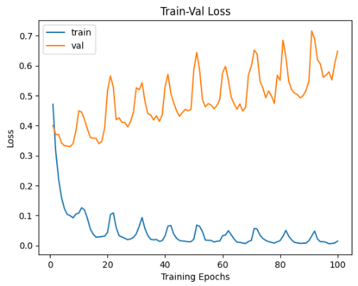
The loss plot
The Metric (Accuracy) Plot
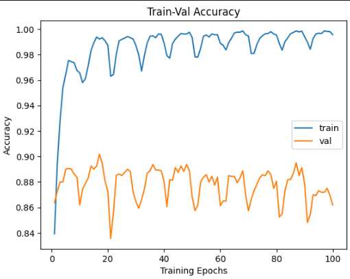
Pretty good if you ask me. You can see the the validation accuracy is around the range of 83% and 90%
Now that we are done with this, we have to make predictions on our test dataset, to do this, we should create a new function to help:
from torch import nn
from torchvision import models

model_resnet = models.resnet18(pretrained=False)
num_ftrs = model_resnet.fc.in_features
num_classes = 10
model_resnet.fc = nn.Linear(num_ftrs, num_classes)
path2weights="./models/resnet18_pretrained.pt"
model_resnet.load_state_dict(torch.load(path2weights))

model_resnet.eval()
if torch.cuda.is_available():
	device = torch.device('cuda')
	model_resnet = model_resnet.to(device)

def deploy_model(model, dataset, device, num_classes=10):
	len_data = len(dataset)
	y_out = torch.zeros(len_data, num_classes)
	y_gt = np.zeros((len_data), dtype='uint8')
	model = model.to(device)
	elapsed_time = []

	with torch.no_grad():
		for i in range(len_data):
			x, y = dataset[i]
			y_gt[i] = y
			start = time.time()
			yy = model(x.unsqueeze(0).to(device))
			y_out[i] = torch.softmax(yy, dim=1)
			elapsed = time.time() - start
			elapsed_time.append(elapsed)

	inference_time=np.mean(elapsed_time)*1000
	print("average inference time per image on %s: %.2f ms "%(device,inference_time))
	return y_out.numpy(),y_gt


y_out,y_gt=deploy_model(model_resnet,test_ds,device=device)
y_pred = np.argmax(y_out,axis=1)
acc=accuracy_score(y_pred,y_gt)
print(acc)
What we have done here is to:
- Load in a new ResNet18 model, and replace the last layer with one that matches our test dataset, like we did earlier, load the weights that we had stored in the
./modelsdirectory, and set the model to evaluation mode. - Next we push the model to the cuda device (GPU) if it is available
- In our
deploy_modelfunction we make predictions for each sample, and return the predictions, along side the true values (the ground truth)
Now we can visualize the model's prediction like so:
from torchvision import utils
%matplotlib inline

np.random.seed(1)

def imshow(inp, title=None):
	mean = [0.4467106, 0.43980986, 0.40664646]
	std = [0.22414584,0.22148906,0.22389975]
	inp = inp.numpy().transpose((1, 2, 0))
	mean = np.array(mean)
	std = np.array(std)
	inp = std * inp + mean
	inp = np.clip(inp, 0, 1)
	plt.imshow(inp)
	if title is not None:
		plt.title(title)
	plt.pause(0.001)

grid_size = 4
rnd_inds = np.random.randint(0, len(test_ds), grid_size)

x_grid_test = [test_ds[i][0] for i in rnd_inds]
y_grid_test = [(y_pred[i], y_gt[i]) for i in rnd_inds]
x_grid_test = utils.make_grid(x_grid_test, nrow=4, padding=2)

plt.rcParams['figure.figsize'] = (10, 5)
imshow(x_grid_test, y_grid_test)
The output should look like:
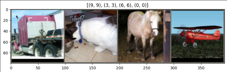
From the plot's title, we can see see that for the selected images, the model made the right prediction.
Well
It has been quite a long journey, but we have finally reached the end : )
Now you might be wondering if this was worth it...
All I can say is; Yes, It was worth it, probably, hopefully, idk lmao
Do have a good one my good sir, and dear lady : )
Tensors
Tensors are basically arrays of numbers. In the context of deep learning, models perform their operations on these array-like objects.
StratifiedShuffleSplit
This is a kind of cross validation splitter in scikit learn that we can use to split datasets and ensure that the class distribution is approximately the same in both splits (in our case, the test_dataset and validate_dataset).
The way (a basic explanation of how) it does this is by taking into account the distributions of class labels, and making sure that both the test dataset and the validate dataset has the same distribution of the class labels (stratifying) and then shuffling the data before it now splits it into the two sets. Hence the name StratifiedShuffleSplit.
More info here
LossFunction
A loss function, to put simply is a function that helps the model know how accurate its predictions are. It is a maths function that measures the difference between the model's predicted value and the actual value. The aim of training the model, is to minimize the loss function, here by increasing the accuracy of the model. Loss functions are super important
Optimizer
An optimizer is a function that assists the model to update its weights, in the right direction, towards predicting values that are more accurate (as compared with the actual values). The optimizer, uses optimization algorithms to minimize the model's loss functions. Optimizers are also super important, and it is important to understand how they work.
LearningRate
Learning rate is a value that determine the magnitude of the updates that is being made to a model's weights during optimization in the training process. A high learning rate value means the magnitude of the changes applied to the model's weights would be large, and vice versa for lower learning rates. Choosing the right learning rate is super important when you want to train a model. An optimal learning rate value is usually derived as experimentation is being carried out.
LearningRateScheduler
A learning rate scheduler is a technique used in training machine learning models to adjust the learning rate during the optimization process. The primary purpose of a learning rate scheduler is to dynamically change the learning rate over the course of training.